graph LR;
    A["basin A"] --- B["basin B"];
    A --- C["basin C"];
    B --- D["basin D"];
    C --- D;
Model concept
A brief summary of the concept is given in the introduction. As indicated, the model concept is organized in three layers:
- a physical layer representing water bodies and associated infrastructure,
- a rule-based control layer to manage the infrastructure, and
- a priority-based allocation layer to take centralized decisions on user_demand abstractions.
1 Physical layer
1.1 Water balance equations
The water balance equation for a drainage basin (Wikipedia contributors 2022) can be defined by a first-order ordinary differential equation (ODE), where the change of the storage \(S\) over time is determined by the inflow fluxes minus the outflow fluxes.
\[ \frac{\mathrm{d}S}{\mathrm{d}t} = Q_{in} - Q_{out} \]
We can split out the fluxes into separate terms, such as precipitation \(P\) and evapotranspiration \(ET\). For now other fluxes are combined into \(Q_{rest}\). If we define all fluxes entering our reservoir as positive, and those leaving the system as negative, all fluxes can be summed up.
\[ \frac{\mathrm{d}S}{\mathrm{d}t} = P + ET + Q_{rest} \]
We don’t use these equations directly. Rather, we use an equivalent formulation where we solve for the cumulative flows instead of the Basin storages. For more details on this see Equations.
1.2 Time
The water balance equation can be applied on many timescales; years, weeks, days or hours. Depending on the application and available data any of these can be the best choice. In Ribasim, we make use of DifferentialEquations.jl and its ODE solvers. Many of these solvers are based on adaptive time stepping, which means the solver will decide how large the time steps can be depending on the state of the system.
The forcing, like precipitation, is generally provided as a time series. Ribasim is set up to support unevenly spaced timeseries. The solver will stop on timestamps where new forcing values are available, so they can be loaded as the new value.
Ribasim is essentially a continuous model, rather than daily or hourly. If you want to use hourly forcing, you only need to make sure that your forcing data contains hourly updates. The output frequency can be configured independently. To be able to write a closed water balance, we accumulate the fluxes. This way any variations in between timesteps are also included, and we can output in m³ rather than m³s⁻¹.
1.3 Space
The water balance equation can be applied on different spatial scales. Besides modeling a single lumped watershed, it allows you to divide the area into a network of connected representative elementary watersheds (REWs) (Reggiani et al. 1998). At this scale global water balance laws can be formulated by means of integration of point-scale conservation equations over control volumes. Such an approach makes Ribasim a semi-distributed model. In this document we typically use the term “basin” to refer to the REW. Each basin has an associated polygon, and the set of basins is connected to each other as described by a graph, which we call the network. Below is a representation of both on the map.
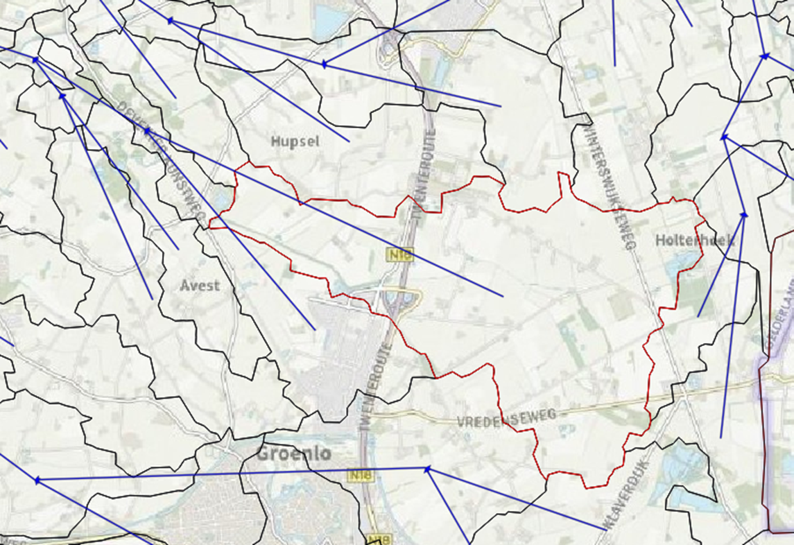
The network is described as graph. Flow can be bi-directional, and the graph does not have to be acyclic.
Internally a directed graph is used. The direction is defined to be the positive flow direction, and is generally set in the dominant flow direction. The basins are the nodes of the network graph. Basin states and properties such storage volume and wetted area are associated with the nodes (A, B, C, D), as are most forcing data such as precipitation, evaporation, or water demand. Basin connection properties and interbasin flows are associated with the links (the lines between A, B, C, and D) instead.
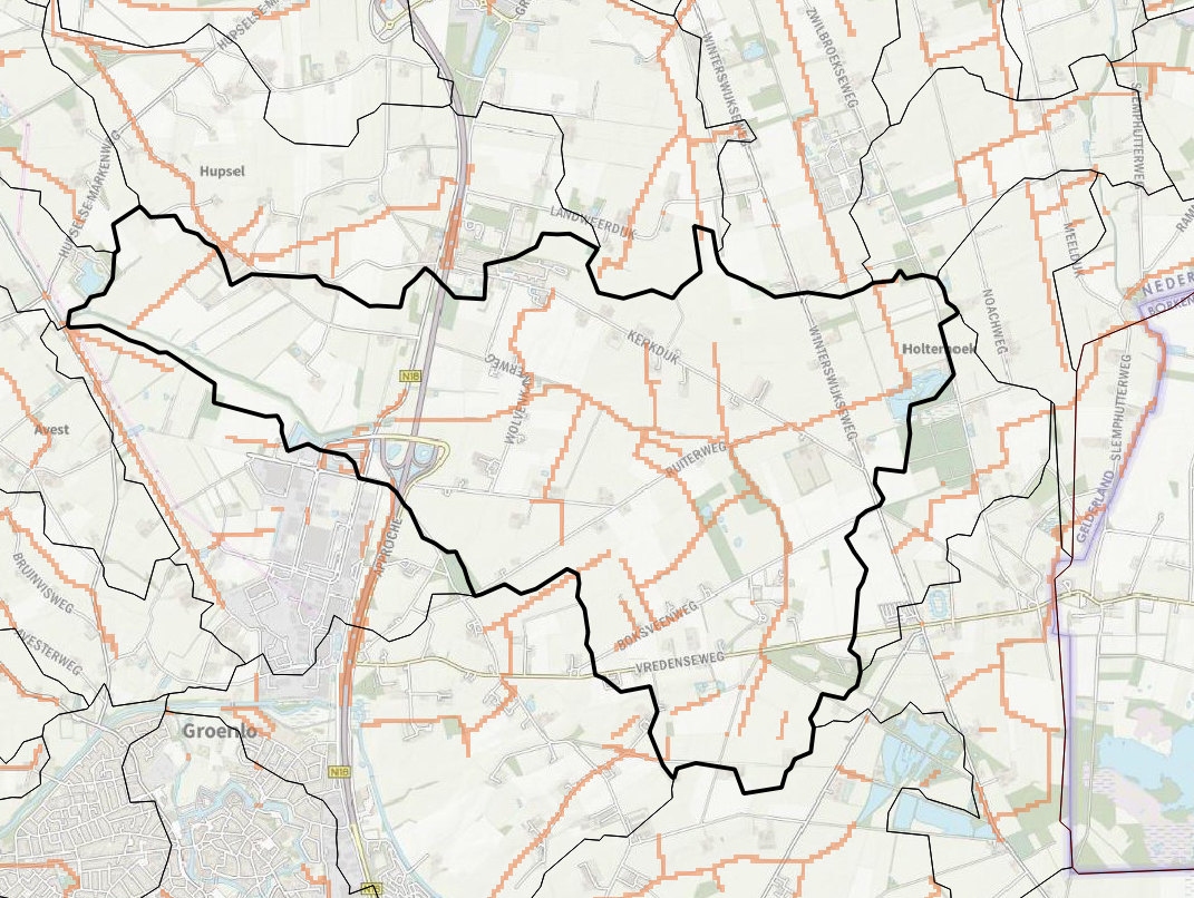
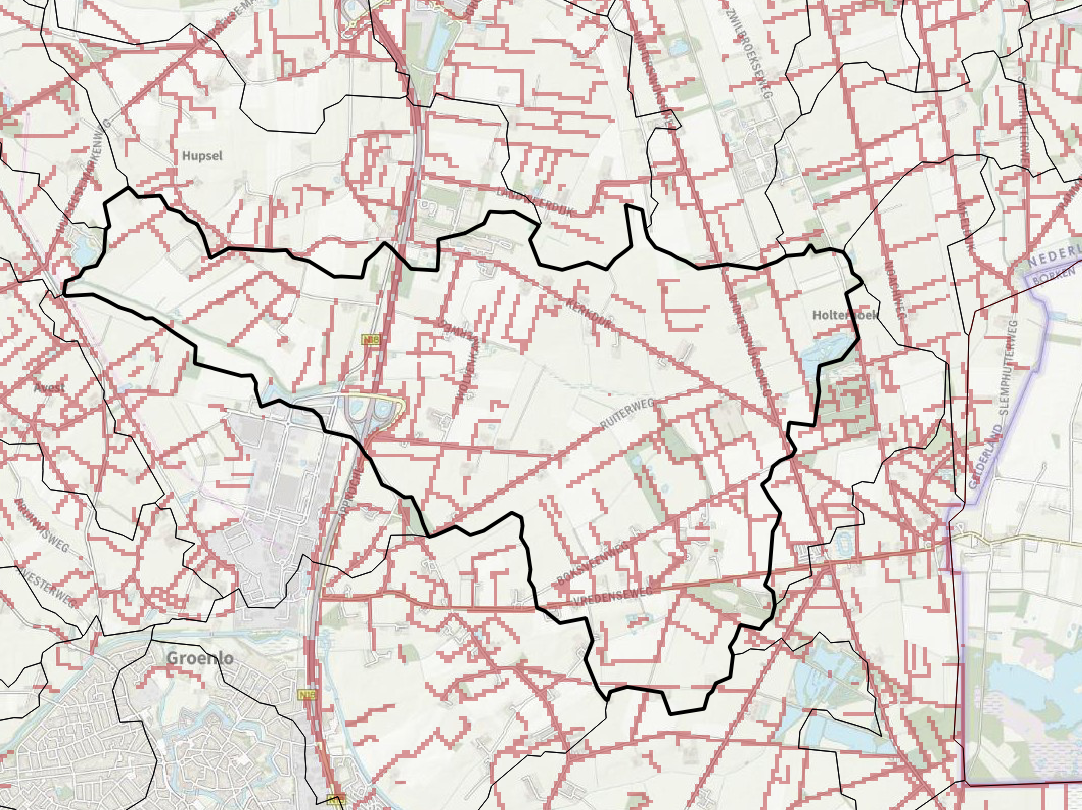
Multiple basins may exist within the same spatial polygon, representing different aspects of the surface water system (perennial ditches, ephemeral ditches, or even surface ponding). Figure 1, Figure 2, Figure 3 show the 25.0 m rasterized primary, secondary, and tertiary surface waters as identified by BRT TOP10NL (PDOK 2022) in the Hupsel basin. These systems may represented in multiple ways.
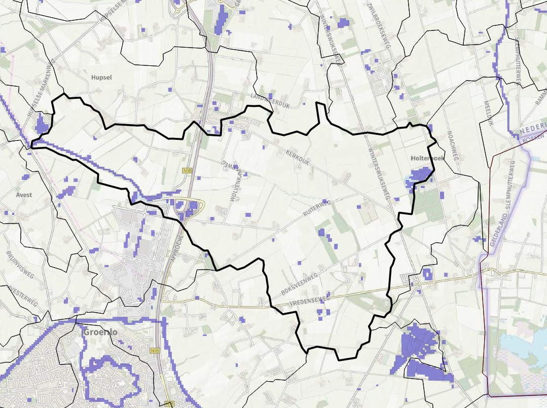
As a single basin (A) containing all surface water, discharging to its downstream basin to the west (B):
graph LR;
    A["basin A"] --> B["basin B"];
Such a system may be capable of representing discharge, but it cannot represent residence times or differences in solute concentrations: within a single basin, a drop of water is mixed instantaneously. Instead, we may group the primary (P), secondary (S), and tertiary (T) surface waters. Then T may flow into S, S into P, and P discharges to the downstream basin (B.)
graph LR;
    T["basin T"] --> S["basin S"];
    S --> P["basin P"];
    P --> B["basin B"];
As each (sub)basin has its own volume, low throughput (high volume, low discharge, long residence time) and high throughput (low volume, high discharge, short residence time) systems can be represented in a lumped manner; of course, more detail requires more parameters.
1.4 Structures in a water system
In addition to free flowing waterbodies, a watersystem typically has structures to control the flow of water. Ribasim uses connector nodes which simplify the hydraulic behavior for the free flowing conditions or structures. The following type of connector nodes are available for this purpose:
- TabulatedRatingCurve: one-directional flow based on upstream head. Node type typically used for gravity flow conditions either free flowing open water channels or over a fixed structure.
- LinearResistance: bi-directional flow based on head difference and linear resistance. Node type typically used for bi-directional flow situations or situations where the head difference over a structure determines its actual flow capacity.
- ManningResistance: bi-directional flow based on head difference and resistance using Manning-Gauckler formula. Same usage as LinearResistance, providing a better hydrological meaning to the resistance parameterization.
- Pump: one-directional structure with a set flow rate. Node type typically used in combination with control to force water over the link.
- Outlet: one-directional gravity structure with a set flow rate. Node type typically used in combination with control to force water over the link, even if there is a mismatch in actual hydraulic capacity. The node type has an automated mechanism to stop the flow when the head difference is zero.
The control layer can activate or deactivate nodes, set flow rates for the Pump and Outlet, or choose different parameterizations for TabulatedRatingCurve, LinearResistance or ManningResistance.
Connector nodes are required within a Ribasim network to determine the flow exchange between basins.
References
PDOK. 2022. Dataset: Basisregistratie Topografie (BRT) TOPNL. https://www.pdok.nl/downloads/-/article/basisregistratie-topografie-brt-topnl.
Reggiani, Paolo, Murugesu Sivapalan, and S. Majid Hassanizadeh. 1998. “A Unifying Framework for Watershed Thermodynamics: Balance Equations for Mass, Momentum, Energy and Entropy, and the Second Law of Thermodynamics.” Advances in Water Resources 22 (4): 367–98. https://doi.org/https://doi.org/10.1016/S0309-1708(98)00012-8.
Wikipedia contributors. 2022. Drainage Basin — Wikipedia, the Free Encyclopedia. https://en.wikipedia.org/w/index.php?title=Drainage_basin&oldid=1099736933.