ManningResistance

The ManningResistance node calculates a flow rate between two Basins based on their water levels. The flow rate is calculated by conservation of energy and the Manning-Gauckler formula to estimate friction losses.

1 Tables

1.1 Static

column	type	unit	restriction
node_id	Int32	-	sorted
control_state	String	-	(optional) sorted per node_id
active	Bool	-	(optional, default true)
length	Float64	\(\text{m}\)	positive
manning_n	Float64	\(\text{s} \text{m}^{-\frac{1}{3}}\)	positive
profile_width	Float64	\(\text{m}\)	positive
profile_slope	Float64	-	-

2 Equations

ManningResistance simulates steady flow between Basins through a reach described by a trapezoidal profile and a Manning roughness coefficient.

We describe the discharge from Basin \(a\) to Basin \(b\) solely as a function of the water levels in \(a\) and \(b\).

\[ Q = f(h_a, h_b) \]

Where:

• The subscripts \(a\) and \(b\) denotes two different Basins
• \(h\) is the hydraulic head, or water level

The energy equation for open channel flow is:

\[ H = h + \frac{v^2}{2g} \]

Where:

• \(H\) is total head
• \(v\) is average water velocity
• \(g\) is gravitational acceleration

The discharge \(Q\) is defined as:

\[ Q = Av \]

where \(A\) is cross-sectional area.

We use conservation of energy to relate the total head at \(a\) to \(b\), with \(H_a > H_b\) as follows:

\[ H_a = H_b + h_{\text{loss}} \]

Or:

\[ h_a + \frac{v_a^2}{2g} = h_b + \frac{v_b^2}{2g} + h_{\text{loss}} \]

Where \(v\) is the average water velocity. \(h_{\text{loss}}\) is a combination of friction and contraction/expansion losses:

\[ h_{\text{loss}} = S_f L + \frac{C}{2g} \left(v_b^2 - v_a^2\right) \]

Where:

• \(L\) is the reach length
• \(S_f\) is the representative friction slope
• \(C\) is the expansion or contraction coefficient, \(0 \le C \le1\)

We assume velocity differences in a connection are negligible (\(v_a = v_b\)):

\[ h_a = h_b + S_f L \]

Friction losses are computed with the Gauckler-Manning formula:

\[ Q = \frac{A}{n} R_h^\frac{2}{3} \sqrt{S_f} \]

Where:

• \(A\) is the representative area.
• \(R_h\) is the representative wetted radius.
• \(S_f\) is the representative friction slope.
• \(n\) is Manning’s roughness coefficient.

We can rewrite to express \(S_f\) in terms of Q:

\[ S_f = Q^2 \frac{n^2}{A^2 R_h^{4/3}} \]

No water is added or removed in a connection:

\[ Q_a = Q_b = Q \]

Substituting:

\[ h_a = h_b + Q^2 \frac{n^2}{A^2 R_h^{4/3}} L \]

We can then express \(Q\) as a function of head difference \(\Delta h\):

\[ Q = \textrm{sign}(\Delta h) \frac{A}{n} R_h^{2/3}\sqrt{\frac{|\Delta h|}{L} } \]

The \(\textrm{sign}(\Delta h)\) term causes the direction of the flow to reverse if the head in basin \(b\) is larger than in basin \(a\).

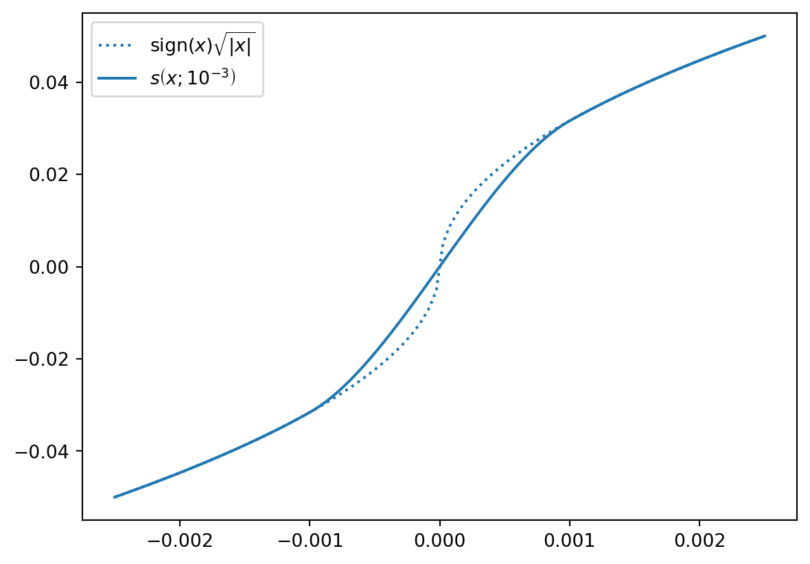
This expression however has a derivative which tends to \(\infty\) as \(\Delta h\) tends to \(0\), which can lead to instabilities in simulation. Therefore we use the modified expression

\[ Q = \frac{A}{n} R_h^{2/3}s\left(\frac{\Delta h}{L}; 10^{-3}\right), \]

where \(s\) is a relaxed square root function:

\[ s(x; x_0) \begin{align} \begin{cases} \frac{x}{4\sqrt{x_0}}\left(5-\left(\frac{x}{x_0}\right)^2\right) &\text{ if } |x| < x_0 \\ \textrm{sign}(x)\sqrt{|x|} &\text{ if } |x| \ge x_0 \end{cases} \end{align} \]

import numpy as np
import matplotlib.pyplot as plt

def s(x, threshold):
  if np.abs(x) < threshold:
    return 1/4 * (x / np.sqrt(threshold)) * (5.0 - (x / threshold)**2)
  else:
    return np.sign(x)*np.sqrt(np.abs(x))

x = np.linspace(-0.0025, 0.0025, 100)
threshold = 1e-3

fig, ax = plt.subplots()

y_o = np.sign(x)*np.sqrt(np.abs(x))
y_s = [s(x_, threshold) for x_ in x]

ax.plot(x, y_o, ls = ":", label = r"sign$(x)\sqrt{|x|}$")
ax.plot(x, y_s, color = "C0", label = r"$s\left(x; 10^{-3}\right)$")
ax.legend()

Note

The computation of \(S_f\) is not exact: we base it on a representative area and hydraulic radius, rather than integrating \(S_f\) along the length of a reach. Direct analytic solutions exist for e.g. parabolic profiles (Tolkmitt), but other profiles requires relatively complicated approaches (such as approximating the profile with a polynomial).

We use the average value of the cross-sectional area, the average value of the water depth, and the average value of the hydraulic radius to compute a friction slope. The size of the resulting error will depend on the water depth difference between the upstream and downstream Basin.

The cross sectional area for a trapezoidal or rectangular profile:

\[ A = w d + \frac{\Delta y}{\Delta z} d^2 \]

Where

• \(w\) is the width at \(d = 0\) (A triangular profile has \(w = 0\))
• \(\frac{\Delta y}{\Delta z}\) is the slope of the profile expressed as the horizontal length for one unit in the vertical (A slope of 45 degrees has \(\frac{\Delta y}{\Delta z} = 1\); a rectangular profile 0).

Accordingly, the wetted perimeter is:

\[ B = w + 2 d \sqrt{\left(\frac{\Delta y}{\Delta z}\right)^2 + 1} \]