from ribasim import run_ribasimIrrigation demand
from pathlib import Path

import matplotlib.pyplot as plt
import pandas as pd
import plotly.express as px
from ribasim import Model, Node
from ribasim.nodes import (
    basin,
    flow_boundary,
    tabulated_rating_curve,
    user_demand,
)
from shapely.geometry import Point
base_dir = Path("crystal-basin")
starttime = "2022-01-01"
endtime = "2023-01-01"
model = Model(
starttime=starttime,
endtime=endtime,
crs="EPSG:4326",
)These nodes are identical to the previous tutorial:
# FlowBoundary
data = pd.DataFrame({
    "time": pd.date_range(start="2022-01-01", end="2023-01-01", freq="MS"),
    "main": [74.7, 57.9, 63.2, 183.9, 91.8, 47.5, 32.6, 27.6, 26.5, 25.1, 39.3, 37.8, 57.9],
    "minor": [16.3, 3.8, 3.0, 37.6, 18.2, 11.1, 12.9, 12.2, 11.2, 10.8, 15.1, 14.3, 11.8]
})  # fmt: skip
data["total"] = data["minor"] + data["main"]
main = model.flow_boundary.add(
    Node(1, Point(0.0, 0.0), name="main"),
    [
        flow_boundary.Time(
            time=data.time,
            flow_rate=data.main,
        )
    ],
)
minor = model.flow_boundary.add(
    Node(2, Point(-3.0, 0.0), name="minor"),
    [
        flow_boundary.Time(
            time=data.time,
            flow_rate=data.minor,
        )
    ],
)

# Basin
confluence = model.basin.add(
    Node(3, Point(-1.5, -1), name="confluence"),
    [
        basin.Profile(area=[672000, 5600000], level=[0, 6]),
        basin.State(level=[4]),
        basin.Time(time=[starttime, endtime]),
    ],
)

# TabulatedRatingCurve
weir = model.tabulated_rating_curve.add(
    Node(4, Point(-1.5, -1.5), name="weir"),
    [
        tabulated_rating_curve.Static(
            level=[0.0, 2, 5],
            flow_rate=[0.0, 50, 200],
        )
    ],
)

# Terminal
sea = model.terminal.add(Node(5, Point(-1.5, -3.0), name="sea"))
1 Irrigation demand
Let us modify the environment to include agricultural activities within the basin, which necessitate irrigation. Water is diverted from the main river through an irrigation canal, with a portion of it eventually returning to the main river (see Figure 1).

For this schematization update, we need to incorporate three additional nodes:
- Basin: Represents a cross-sectional point where water is diverted.
- UserDemand: Represents the irrigation demand.
- TabulatedRatingCurve: Defines the remaining water flow from the main river at the diversion point.
1.1 Add a second Basin node
This Basin will portray as the point in the river where the diversion takes place, getting the name diversion. Its profile area at this intersection is slightly smaller than at the confluence.
diversion_basin = model.basin.add(
    Node(6, Point(-0.75, -0.5), name="diversion_basin"),
    [
        basin.Profile(area=[500000, 5000000], level=[0, 6]),
        basin.State(level=[3]),
        basin.Time(time=[starttime, endtime]),
    ],
)
1.2 Add the irrigation demand
An irrigation district needs to apply irrigation to its field starting from April to September. The irrigated area is \(> 17000 \text{ ha}\) and requires around \(5 \text{ mm/day}\). In this case the irrigation district diverts from the main river an average flow rate of \(10 \text{ m}^3/\text{s}\) and \(12 \text{ m}^3/\text{s}\) during spring and summer, respectively. Start of irrigation takes place on the 1st of April until the end of September. The water intake is through a canal (demand).
For now, let’s assume the return flow remains \(0.0\) (return_factor). Meaning all the supplied water to fulfill the demand is consumed and does not return back to the river. The user demand node interpolates the demand values. Thus the following code needs to be implemented:
irrigation = model.user_demand.add(
    Node(7, Point(-1.5, 0.5), name="irrigation"),
    [
        user_demand.Time(
            demand=[0.0, 0.0, 10, 12, 12, 0.0],
            return_factor=0,
            min_level=0,
            demand_priority=1,
            time=[
                starttime,
                "2022-03-31",
                "2022-04-01",
                "2022-07-01",
                "2022-09-30",
                "2022-10-01",
            ],
        )
    ],
)
1.3 Add a TabulatedRatingCurve
The second TabulatedRatingCurve node will simulate the rest of the water that is left after diverting a part from the main river to the irrigation disctrict. The rest of the water will flow naturally towards the confluence:
diversion_weir = model.tabulated_rating_curve.add(
    Node(8, Point(-1.125, -0.75), name="diversion_weir"),
    [
        tabulated_rating_curve.Static(
            level=[0.0, 1.5, 5],
            flow_rate=[0.0, 45, 200],
        )
    ],
)
1.4 Add links
model.link.add(main, diversion_basin, name="main")
model.link.add(minor, confluence, name="minor")
model.link.add(diversion_basin, irrigation, name="irrigation")
model.link.add(irrigation, confluence)
model.link.add(diversion_basin, diversion_weir, name="not diverted")
model.link.add(diversion_weir, confluence)
model.link.add(confluence, weir)
model.link.add(weir, sea, name="sea")
toml_path = base_dir / "Crystal-2/ribasim.toml"
model.write(toml_path)
cli_path = "ribasim"1.5 Plot model and run
Plot the schematization and run the model. This time the new outputs should be written in a new folder called Crystal-2:
model.plot();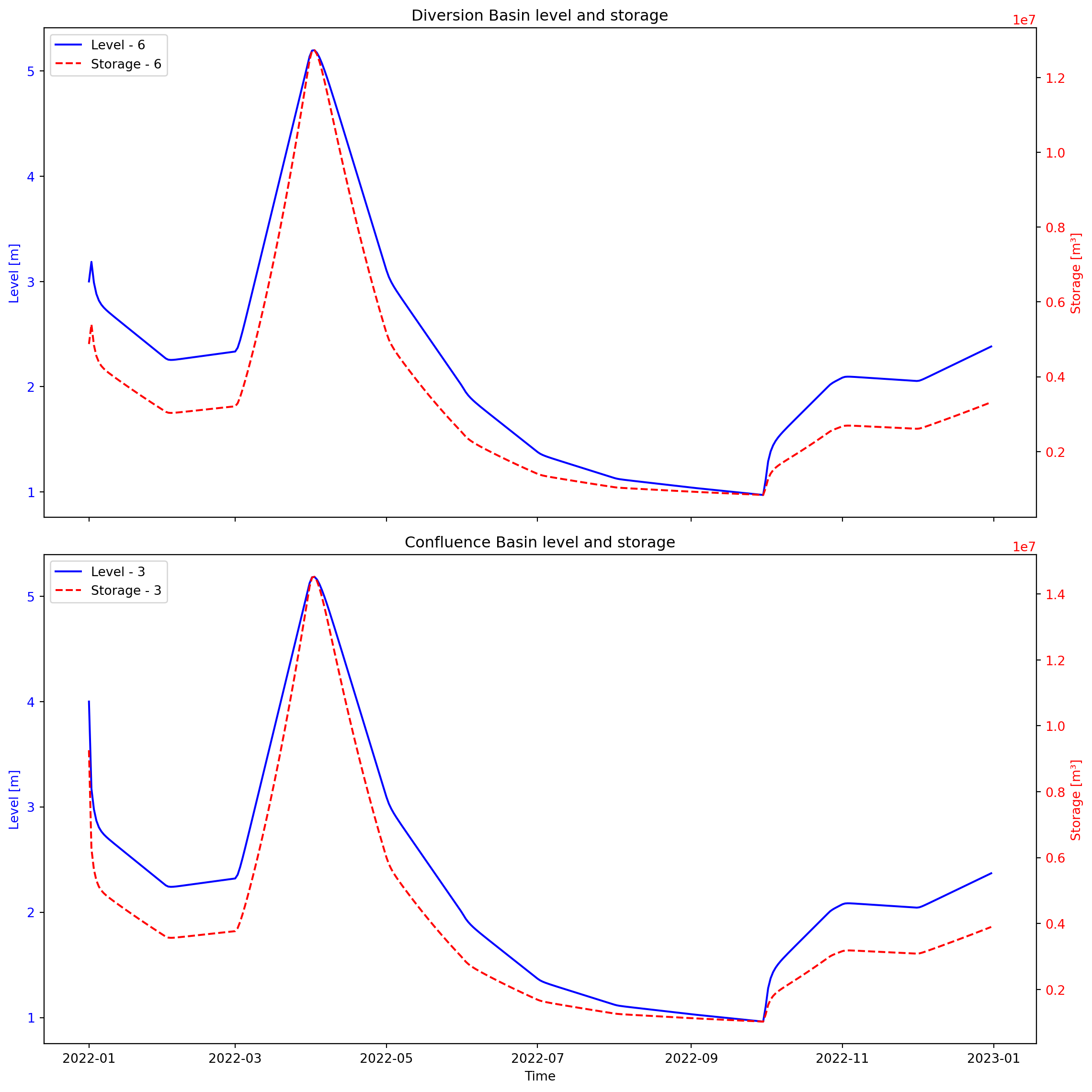
run_ribasim(toml_path)┌ Info: Starting a Ribasim simulation.
│ toml_path = "crystal-basin/Crystal-2/ribasim.toml"
│ cli.ribasim_version = "2025.6.0"
│ starttime = 2022-01-01T00:00:00
│ endtime = 2023-01-01T00:00:00
└ threads = 1
Simulating 0%| | ETA: N/A
Simulating 0%| | ETA: 16:36:45
Simulating 2%|▉ | ETA: 0:26:14
Simulating 9%|███▍ | ETA: 0:06:20
Simulating 12%|████▉ | ETA: 0:04:18
Simulating 17%|██████▊ | ETA: 0:02:55
Simulating 25%|█████████▊ | ETA: 0:01:49
Simulating 25%|█████████▉ | ETA: 0:01:48
Simulating 25%|█████████▉ | ETA: 0:01:48
Simulating 25%|█████████▉ | ETA: 0:01:48
Simulating 25%|█████████▉ | ETA: 0:01:48
Simulating 25%|██████████ | ETA: 0:01:46
Simulating 28%|███████████▏ | ETA: 0:01:32
Simulating 33%|█████████████▏ | ETA: 0:01:12
Simulating 37%|██████████████▋ | ETA: 0:01:01
Simulating 42%|████████████████▊ | ETA: 0:00:50
Simulating 47%|██████████████████▊ | ETA: 0:00:40
Simulating 50%|███████████████████▉ | ETA: 0:00:36
Simulating 51%|████████████████████▎ | ETA: 0:00:35
Simulating 58%|███████████████████████▎ | ETA: 0:00:26
Simulating 61%|████████████████████████▌ | ETA: 0:00:23
Simulating 68%|███████████████████████████▎ | ETA: 0:00:17
Simulating 75%|█████████████████████████████▉ | ETA: 0:00:12
Simulating 75%|█████████████████████████████▉ | ETA: 0:00:12
Simulating 75%|██████████████████████████████ | ETA: 0:00:12
Simulating 82%|████████████████████████████████▉ | ETA: 0:00:08
Simulating 84%|█████████████████████████████████▋ | ETA: 0:00:07
Simulating 92%|████████████████████████████████████▋ | ETA: 0:00:03
Simulating 95%|█████████████████████████████████████▉ | ETA: 0:00:02
Simulating 100%|████████████████████████████████████████| Time: 0:00:35
[ Info: Computation time: 16 seconds, 538 milliseconds
[ Info: The model finished successfully.1.6 Plot and compare the Basin results
Plot the simulated levels and storages at the diverted section and at the confluence.
df_basin = pd.read_feather(base_dir / "Crystal-2/results/basin.arrow")

# Create pivot tables and plot for basin data
df_basin_wide = df_basin.pivot_table(
    index="time", columns="node_id", values=["storage", "level"]
)

df_basin_div = df_basin_wide.loc[:, pd.IndexSlice[:, diversion_basin.node_id]]
df_basin_conf = df_basin_wide.loc[:, pd.IndexSlice[:, confluence.node_id]]


def plot_basin_data(
    ax, ax_twin, df_basin, level_color="b", storage_color="r", title="Basin"
):
    # Plot level data
    for column in df_basin["level"].columns:
        ax.plot(
            df_basin.index,
            df_basin["level"][column],
            linestyle="-",
            color=level_color,
            label=f"Level - {column}",
        )

    # Plot storage data
    for column in df_basin["storage"].columns:
        ax_twin.plot(
            df_basin.index,
            df_basin["storage"][column],
            linestyle="--",
            color=storage_color,
            label=f"Storage - {column}",
        )

    ax.set_ylabel("Level [m]", color=level_color)
    ax_twin.set_ylabel("Storage [m³]", color=storage_color)

    ax.tick_params(axis="y", labelcolor=level_color)
    ax_twin.tick_params(axis="y", labelcolor=storage_color)

    ax.set_title(title)

    # Combine legends from both axes
    lines, labels = ax.get_legend_handles_labels()
    lines_twin, labels_twin = ax_twin.get_legend_handles_labels()
    ax.legend(lines + lines_twin, labels + labels_twin, loc="upper left")


# Create subplots
fig, (ax1, ax3) = plt.subplots(2, 1, figsize=(12, 12), sharex=True)

# Plot Div basin data
ax2 = ax1.twinx()  # Secondary y-axis for storage
plot_basin_data(ax1, ax2, df_basin_div, title="Diversion Basin level and storage")

# Plot Conf basin data
ax4 = ax3.twinx()  # Secondary y-axis for storage
plot_basin_data(ax3, ax4, df_basin_conf, title="Confluence Basin level and storage")

# Common X label
ax3.set_xlabel("Time")
fig.tight_layout()  # Adjust layout to fit labels
plt.show()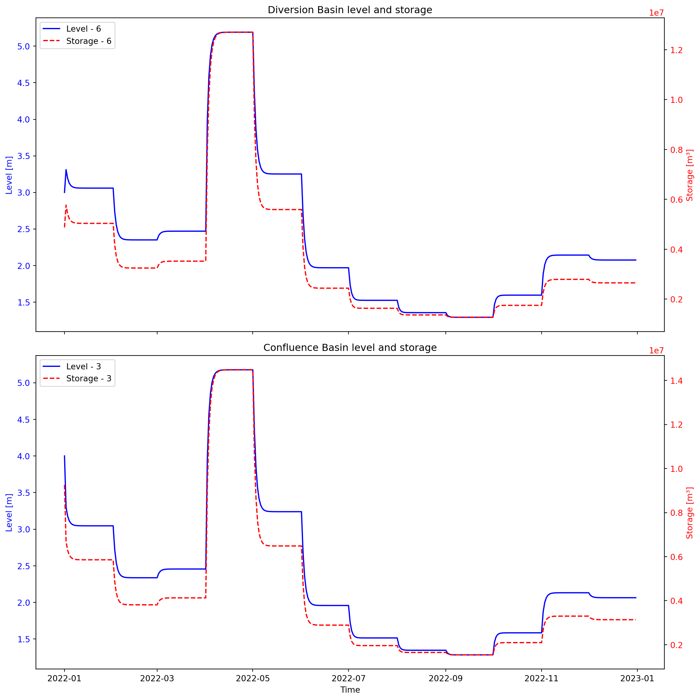
The figure above illustrates the water levels and storage capacities for each Basin.
When compared to the natural flow conditions, where no water is abstracted for irrigation (See Crystal 1), there is a noticeable decrease in both storage and water levels at the confluence downstream. This reduction is attributed to the irrigation demand upstream with no return flow, which decreases the amount of available water in the main river, resulting in lower water levels at the confluence.
1.7 Plot and compare the flow results
Plot the flow results in an interactive plotting tool.
df_flow = pd.read_feather(base_dir / "Crystal-2/results/flow.arrow")
# Add the link names and then remove unnamed links
df_flow["name"] = model.link.df["name"].loc[df_flow["link_id"]].to_numpy()
df_flow = df_flow[df_flow["name"].astype(bool)]

# Plot the flow data, interactive plot with Plotly
pivot_flow = df_flow.pivot_table(
    index="time", columns="name", values="flow_rate"
).reset_index()
fig = px.line(pivot_flow, x="time", y=pivot_flow.columns[1:], title="Flow [m3/s]")

fig.update_layout(legend_title_text="Link")
fig.show()
Try toggling the links on and off by clicking on them in the links.