from pathlib import Path

import matplotlib.pyplot as plt
import pandas as pd
import plotly.express as px
import xarray as xr
from ribasim import Model, Node, run_ribasim
from ribasim.nodes import (
    basin,
    flow_boundary,
    tabulated_rating_curve,
    user_demand,
)
from shapely.geometry import PointReservoir
base_dir = Path("crystal-basin")

starttime = "2022-01-01"
endtime = "2023-01-01"
model = Model(
    starttime=starttime,
    endtime=endtime,
    crs="EPSG:4326",
)
These nodes are identical to the previous tutorial:
# FlowBoundary
data = pd.DataFrame({
    "time": pd.date_range(start="2022-01-01", end="2023-01-01", freq="MS"),
    "main": [74.7, 57.9, 63.2, 183.9, 91.8, 47.5, 32.6, 27.6, 26.5, 25.1, 39.3, 37.8, 57.9],
    "minor": [16.3, 3.8, 3.0, 37.6, 18.2, 11.1, 12.9, 12.2, 11.2, 10.8, 15.1, 14.3, 11.8]
})  # fmt: skip
data["total"] = data["minor"] + data["main"]
main = model.flow_boundary.add(
    Node(1, Point(0.0, 0.0), name="main"),
    [
        flow_boundary.Time(
            time=data.time,
            flow_rate=data.main,
        )
    ],
)
minor = model.flow_boundary.add(
    Node(2, Point(-3.0, 0.0), name="minor"),
    [
        flow_boundary.Time(
            time=data.time,
            flow_rate=data.minor,
        )
    ],
)

# Basin
confluence = model.basin.add(
    Node(3, Point(-1.5, -1), name="confluence"),
    [
        basin.Profile(area=[672000, 5600000], level=[0, 6]),
        basin.State(level=[4]),
        basin.Time(time=[starttime, endtime]),
    ],
)

# TabulatedRatingCurve
weir = model.tabulated_rating_curve.add(
    Node(4, Point(-1.5, -1.5), name="weir"),
    [
        tabulated_rating_curve.Static(
            level=[0.0, 2, 5],
            flow_rate=[0.0, 50, 200],
        )
    ],
)
diversion_weir = model.tabulated_rating_curve.add(
    Node(8, Point(-1.125, -0.75), name="diversion_weir"),
    [
        tabulated_rating_curve.Static(
            level=[0.0, 1.5, 5],
            flow_rate=[0.0, 45, 200],
        )
    ],
)

# UserDemand
irrigation = model.user_demand.add(
    Node(7, Point(-1.5, 0.5), name="irrigation"),
    [
        user_demand.Time(
            demand=[0.0, 0.0, 10, 12, 12, 0.0],
            return_factor=0,
            min_level=0,
            demand_priority=1,
            time=[
                starttime,
                "2022-03-31",
                "2022-04-01",
                "2022-07-01",
                "2022-09-30",
                "2022-10-01",
            ],
        )
    ],
)

# Terminal
sea = model.terminal.add(Node(5, Point(-1.5, -3.0), name="sea"))
Due to the increase of population and climate change Crystal city has implemented a reservoir upstream to store water for domestic use (See Figure 1). The reservoir is to help ensure a reliable supply during dry periods. In this module, the user will update the model to incorporate the reservoir’s impact on the whole Crystal basin.

1 Reservoir
1.1 Add a Basin
The diversion_basin from the previous tutorial is not used, but replaced by a larger reservoir Basin. Its water will play an important role for the users (the city and the irrigation district). The reservoir has a maximum area of \(32.3 \text{ km}^2\) and a maximum depth of \(7 \text{ m}\).
reservoir = model.basin.add(
    Node(6, Point(-0.75, -0.5), name="reservoir"),
    [
        basin.Profile(area=[20000000, 32300000], level=[0, 7]),
        basin.State(level=[3.5]),
        basin.Time(time=[starttime, endtime]),
    ],
)
1.2 Add a demand node
\(50.000\) people live in Crystal City. To represents the total flow rate or abstraction rate required to meet the water demand of \(50.000\) people, another demand node needs to be added assuming a return flow of \(60\%\).
city = model.user_demand.add(
    Node(9, Point(0, -1), name="city"),
    [
        user_demand.Time(
            # Total demand in m³/s
            demand=[0.07, 0.08, 0.09, 0.10, 0.12, 0.14, 0.15, 0.14, 0.12, 0.10, 0.09, 0.08],
            return_factor=0.6,
            min_level=0,
            demand_priority=1,
            time=pd.date_range(start="2022-01-01", periods=12, freq="MS"),
        )
    ],
)  # fmt: skip
model.link.add(main, reservoir, name="main")
model.link.add(minor, confluence, name="minor")
model.link.add(reservoir, irrigation, name="irrigation")
model.link.add(irrigation, confluence)
model.link.add(reservoir, city, name="city")
model.link.add(city, confluence, name="city returnflow")
model.link.add(reservoir, diversion_weir, name="not diverted")
model.link.add(diversion_weir, confluence)
model.link.add(confluence, weir)
model.link.add(weir, sea, name="sea")model.plot();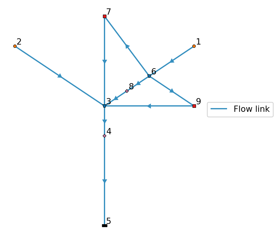
toml_path = base_dir / "Crystal-3/ribasim.toml"
model.write(toml_path)PosixPath('crystal-basin/Crystal-3/ribasim.toml')1.3 Adjust the code
Adjust the naming of the Basin in the dictionary mapping and the saving file should be Crystal-3.
run_ribasim(toml_path)⠀⠀⠀⠀⠀⠀⠀⣿⣿⢂⣀⠀⠀⠀⠀⠀⠀⠀⠀⠀
⠀⠀⠀⠀⠀⠀⣾⣶⣶⣿⡿⢟⣴⣶⡆⣾⣿⡆⠀⠀
⠀⢀⣀⢠⣶⣷⢻⡇⠀⢀⣄⠟⠉⠙⢿⣮⣭⠀⠀⠀
⠀⢿⣿⢇⣿⠃⠈⠃⣰⣿⣿⣧⠀⣠⣈⣛⠿⠀⠀⠀ Ribasim v2026.1.2
⠀⠀⠰⣿⣧⣀⠀⠰⣿⣿⣿⣿⡇⠀⠈⢹⣿⡦⠀⠀ Water resources modeling
⠀⠀⠀⢰⣮⣍⠉⠁⠙⠻⠿⠛⠐⡄⢠⣾⡏⣾⣿⡆
⠀⠀⠀⢘⣛⢿⣆⣀⣠⡞⠀⠀⠀⣿⣸⠿⠗⠈⠉⠀
⠀⠀⠀⢿⣿⠇⠿⠟⢿⣾⣿⠿⠿⠿⠃⠀⠀⠀⠀⠀
⠀⠀⠀⠀⠀⠀⠀⠀⠀⠈⠁⣿⣿⠆⠀⠀⠀⠀⠀⠀
┌ Info: Starting a Ribasim simulation at 2026-10-02T17:57:02.996.
│ toml_path = "crystal-basin/Crystal-3/ribasim.toml"
│ ribasim_version = "2026.1.2"
│ ribasim_home = "/home/runner/work/Ribasim/Ribasim/.pixi/envs/default"
│ starttime = 2022-01-01T00:00:00
│ endtime = 2023-01-01T00:00:00
└ threads = 1
Simulating 0%| | ETA: N/A
Simulating 0%| | ETA: 4:18:44
Simulating 8%|███▍ | ETA: 0:01:37
Simulating 11%|████▎ | ETA: 0:01:15
Simulating 16%|██████▌ | ETA: 0:00:47
Simulating 25%|█████████▉ | ETA: 0:00:27
Simulating 25%|█████████▉ | ETA: 0:00:28
Simulating 33%|█████████████▏ | ETA: 0:00:18
Simulating 33%|█████████████▎ | ETA: 0:00:18
Simulating 41%|████████████████▌ | ETA: 0:00:13
Simulating 47%|██████████████████▋ | ETA: 0:00:10
Simulating 50%|███████████████████▉ | ETA: 0:00:09
Simulating 58%|███████████████████████▎ | ETA: 0:00:07
Simulating 67%|██████████████████████████▋ | ETA: 0:00:05
Simulating 69%|███████████████████████████▊ | ETA: 0:00:04
Simulating 75%|█████████████████████████████▉ | ETA: 0:00:03
Simulating 83%|█████████████████████████████████▏ | ETA: 0:00:02
Simulating 86%|██████████████████████████████████▍ | ETA: 0:00:01
Simulating 92%|████████████████████████████████████▋ | ETA: 0:00:01
Simulating 100%|████████████████████████████████████████| Time: 0:00:09
[ Info: Computation time: 9 seconds, 45 milliseconds
[ Info: Writing results.
┌ Info: Convergence bottlenecks in descending order of severity (1.0 is the
│ worst):
│ TabulatedRatingCurve #8 = 1.0
└ TabulatedRatingCurve #4 = 0.8
[ Info: The model finished successfully at 2026-10-02T17:58:11.877.2 Plot reservoir storage and level
ds_basin = xr.open_dataset(base_dir / "Crystal-3/results/basin.nc")
df_basin = ds_basin.to_dataframe().reset_index()

# Create pivot tables and plot for Basin data
df_basin_wide = df_basin.pivot_table(
    index="time", columns="node_id", values=["storage", "level"]
)
df_basin_wide = df_basin_wide.loc[:, pd.IndexSlice[:, reservoir.node_id]]

# Plot level and storage on the same graph with dual y-axes
fig, ax1 = plt.subplots(figsize=(12, 6))

# Plot level on the primary y-axis
color = "b"
ax1.set_xlabel("Time")
ax1.set_ylabel("Level [m]", color=color)
ax1.plot(df_basin_wide.index, df_basin_wide["level"], color=color)
ax1.tick_params(axis="y", labelcolor=color)

# Create a secondary y-axis for storage
ax2 = ax1.twinx()
color = "r"
ax2.set_ylabel("Storage [m³]", color="r")
ax2.plot(df_basin_wide.index, df_basin_wide["storage"], linestyle="--", color=color)
ax2.tick_params(axis="y", labelcolor=color)

fig.tight_layout()  # Adjust layout to fit labels
plt.title("Basin level and storage")
plt.show()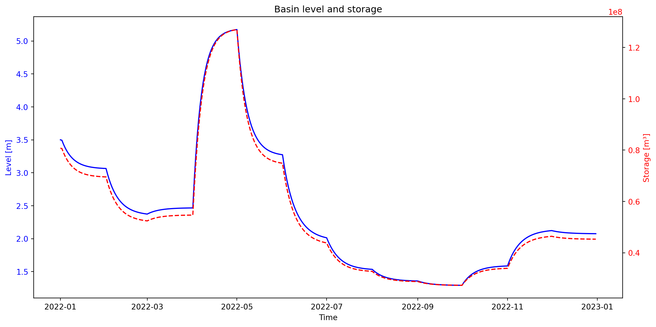
The figure above illustrates the storage and water level at the reservoir. As expected, after increasing the profile of the Basin, its storage capacity increased as well.
3 Plot flows
ds_flow = xr.open_dataset(base_dir / "Crystal-3/results/flow.nc")
df_flow = ds_flow.to_dataframe().reset_index()
# Add the link names and then remove unnamed links
df_flow["name"] = model.link.df["name"].loc[df_flow["link_id"]].to_numpy()
df_flow = df_flow[df_flow["name"].astype(bool)]

# Plot the flow data, interactive plot with Plotly
pivot_flow = df_flow.pivot_table(
    index="time", columns="name", values="flow_rate"
).reset_index()
fig = px.line(pivot_flow, x="time", y=pivot_flow.columns[1:], title="Flow [m3/s]")

fig.update_layout(legend_title_text="Link")
fig.show()