Ribasim Delwaq coupling

In order to generate the Delwaq input files, we need a completed Ribasim simulation (typically one with a results folder) that ideally also includes some substances and initial concentrations. Let’s take the basic test model for example, which already has set some initial concentrations.

All testmodels can be downloaded from here.

1 Generating Delwaq input

from pathlib import Path

toml_path = Path("../../generated_testmodels/basic/ribasim.toml")

This Ribasim model already has substance concentrations for Cl and Tracer in the input tables, and we will use these to generate the Delwaq input files.

from ribasim import Model, run_ribasim

model = Model.read(toml_path)

display(model.basin.concentration_state)  # basin initial state
display(model.basin.concentration)  # basin boundaries
display(model.flow_boundary.concentration)  # flow boundaries
display(model.level_boundary.concentration)  # level boundaries
model.plot();  # for later comparison

Basin / concentration_state

	node_id	substance	concentration
fid
0	1	Cl	0.0
1	3	Cl	0.0
2	6	Cl	0.0
3	9	Cl	0.0

Basin / concentration

	node_id	time	substance	drainage	precipitation	surface_runoff
fid
0	1	2020-01-01	Cl	0.0	0.0	0.0
1	1	2020-01-02	Cl	1.0	1.0	1.0
2	1	2020-01-01	Tracer	1.0	1.0	1.0
3	3	2020-01-01	Cl	0.0	0.0	0.0
4	3	2020-01-02	Cl	1.0	1.0	1.0
5	3	2020-01-01	Tracer	1.0	1.0	1.0
6	6	2020-01-01	Cl	0.0	0.0	0.0
7	6	2020-01-02	Cl	1.0	1.0	1.0
8	6	2020-01-01	Tracer	1.0	1.0	1.0
9	9	2020-01-01	Cl	0.0	0.0	0.0
10	9	2020-01-02	Cl	1.0	1.0	1.0
11	9	2020-01-01	Tracer	1.0	1.0	1.0

FlowBoundary / concentration

	node_id	time	substance	concentration
fid
0	15	2020-01-01	Cl	0.0
1	15	2020-01-01	Tracer	1.0
2	16	2020-01-01	Cl	0.0
3	16	2020-01-01	Tracer	1.0

LevelBoundary / concentration

	node_id	time	substance	concentration
fid
0	11	2020-01-01	Cl	34.0
1	17	2020-01-01	Cl	34.0

model.basin.profile

Basin / profile

	node_id	area	level	storage
fid
0	1	0.01	0.0	NaN
1	1	1000.00	1.0	NaN
2	3	0.01	0.0	NaN
3	3	1000.00	1.0	NaN
4	6	0.01	0.0	NaN
5	6	1000.00	1.0	NaN
6	9	0.01	0.0	NaN
7	9	1000.00	1.0	NaN

Let’s add another tracer to the model, to setup a fraction calculation.

from ribasim.delwaq import add_tracer

add_tracer(model, 11, "Foo")
add_tracer(model, 15, "Bar")
display(model.flow_boundary.concentration)  # flow boundaries
display(model.level_boundary.concentration)  # flow boundaries

model.write(toml_path)

FlowBoundary / concentration

	node_id	time	substance	concentration
fid
0	15	2020-01-01	Cl	0.0
1	15	2020-01-01	Tracer	1.0
2	16	2020-01-01	Cl	0.0
3	16	2020-01-01	Tracer	1.0
4	15	2020-01-01	Bar	1.0

LevelBoundary / concentration

	node_id	time	substance	concentration
fid
0	11	2020-01-01	Cl	34.0
1	17	2020-01-01	Cl	34.0
2	11	2020-01-01	Foo	1.0

PosixPath('../../generated_testmodels/basic/ribasim.toml')

run_ribasim(toml_path)

⠀⠀⠀⠀⠀⠀⠀⣿⣿⢂⣀⠀⠀⠀⠀⠀⠀⠀⠀⠀

⠀⠀⠀⠀⠀⠀⣾⣶⣶⣿⡿⢟⣴⣶⡆⣾⣿⡆⠀⠀

⠀⢀⣀⢠⣶⣷⢻⡇⠀⢀⣄⠟⠉⠙⢿⣮⣭⠀⠀⠀

⠀⢿⣿⢇⣿⠃⠈⠃⣰⣿⣿⣧⠀⣠⣈⣛⠿⠀⠀⠀  Ribasim v2026.1.0-rc2

⠀⠀⠰⣿⣧⣀⠀⠰⣿⣿⣿⣿⡇⠀⠈⢹⣿⡦⠀⠀  Water resources modeling

⠀⠀⠀⢰⣮⣍⠉⠁⠙⠻⠿⠛⠐⡄⢠⣾⡏⣾⣿⡆

⠀⠀⠀⢘⣛⢿⣆⣀⣠⡞⠀⠀⠀⣿⣸⠿⠗⠈⠉⠀

⠀⠀⠀⢿⣿⠇⠿⠟⢿⣾⣿⠿⠿⠿⠃⠀⠀⠀⠀⠀

⠀⠀⠀⠀⠀⠀⠀⠀⠀⠈⠁⣿⣿⠆⠀⠀⠀⠀⠀⠀



┌ Info: Starting a Ribasim simulation at 2026-03-17T09:27:52.209.

│   toml_path = "../../generated_testmodels/basic/ribasim.toml"

│   ribasim_version = "2026.1.0-rc2"

│   ribasim_home = "/home/runner/.julia/juliaup/julia-1.12.5+0.x64.linux.gnu"

│   starttime = 2020-01-01T00:00:00

│   endtime = 2021-01-01T00:00:00

└   threads = 1

┌ Warning: The following experimental features are enabled: concentration

└ @ Ribasim /home/runner/work/Ribasim/Ribasim/core/src/logging.jl:56

Simulating   0%|                                        |  ETA: N/A

Simulating   6%|██▎                                     |  ETA: 0:03:01

Simulating  33%|█████████████▎                          |  ETA: 0:00:22

Simulating  60%|████████████████████████▏               |  ETA: 0:00:07

Simulating  88%|███████████████████████████████████▏    |  ETA: 0:00:02

Simulating 100%|████████████████████████████████████████| Time: 0:00:11

[ Info: Computation time: 8 seconds, 182 milliseconds

[ Info: Writing results.

[ Info: The model finished successfully at 2026-03-17T09:28:44.284.

Given the path to a completed Ribasim simulation, we can call ribasim.delwaq.generate for generating the required input files for Delwaq from scratch. ribasim.delwaq.generate either takes a Model instance, or the path to a toml file, as well as an output_path keyword, where the input for Delwaq will be written. By default it is set to the delwaq folder next to the toml.

from ribasim.delwaq import generate

# The default path is the delwaq folder next to the toml
output_path = Path("../../generated_testmodels/basic/delwaq")

graph, substances = generate(model, output_path)

/home/runner/work/Ribasim/Ribasim/python/ribasim/ribasim/delwaq/generate.py:504: SettingWithCopyWarning: 
A value is trying to be set on a copy of a slice from a DataFrame.
Try using .loc[row_indexer,col_indexer] = value instead

See the caveats in the documentation: https://pandas.pydata.org/pandas-docs/stable/user_guide/indexing.html#returning-a-view-versus-a-copy
  volumes["riba_node_id"] = volumes.loc[:, "node_id"]

This call produces a handful of files in the user defined folder. Let’s take a look at them:

list(output_path.iterdir())

[PosixPath('../../generated_testmodels/basic/delwaq/B8_initials.inc'),
 PosixPath('../../generated_testmodels/basic/delwaq/B6_wasteloads.inc'),
 PosixPath('../../generated_testmodels/basic/delwaq/ribasim.nc'),
 PosixPath('../../generated_testmodels/basic/delwaq/B5_bounddata.inc'),
 PosixPath('../../generated_testmodels/basic/delwaq/ribasim.vel'),
 PosixPath('../../generated_testmodels/basic/delwaq/delwaq.inp'),
 PosixPath('../../generated_testmodels/basic/delwaq/dimr_config.xml'),
 PosixPath('../../generated_testmodels/basic/delwaq/ribasim.poi'),
 PosixPath('../../generated_testmodels/basic/delwaq/ribasim.len'),
 PosixPath('../../generated_testmodels/basic/delwaq/network.csv'),
 PosixPath('../../generated_testmodels/basic/delwaq/ribasim.atr'),
 PosixPath('../../generated_testmodels/basic/delwaq/ribasim.are'),
 PosixPath('../../generated_testmodels/basic/delwaq/ribasim.flo'),
 PosixPath('../../generated_testmodels/basic/delwaq/bndlist.csv'),
 PosixPath('../../generated_testmodels/basic/delwaq/ribasim.vol'),
 PosixPath('../../generated_testmodels/basic/delwaq/ribasim_bndlist.inc')]

These files form a complete Delwaq simulation, and can be run by either pointing DIMR to the dimr_config.xml file or pointing Delwaq to the delwaq.inp file.

Note that the call to generate produces two output variables; graph and substances that are required for parsing the results of the Delwaq model later on. Nonetheless, we can also inspect them here, and inspect the created Delwaq network.

substances  # list of substances, as will be present in the Delwaq netcdf output

{'Bar',
 'Cl',
 'Continuity',
 'Drainage',
 'FlowBoundary',
 'Foo',
 'Initial',
 'LevelBoundary',
 'Precipitation',
 'SurfaceRunoff',
 'Tracer',
 'UserDemand'}

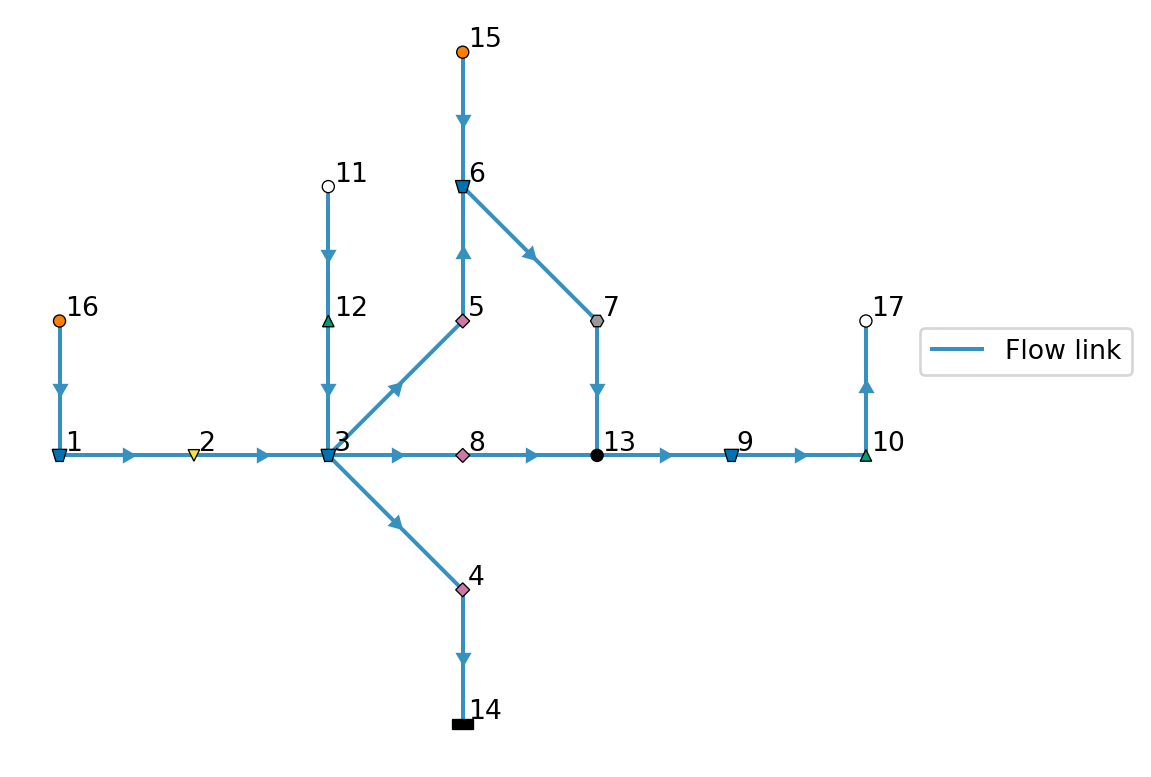
As you can see, the complete substances list is a combination of user input (Cl and Tracer in the input tables), a Continuity tracer, and tracers for all nodetypes in the Ribasim model. The latter tracers allow for deeper inspection of the Ribasim model, such as debugging the mass balance by plotting fraction graphs. Let’s inspect the graph next, which is the Delwaq network that was created from the Ribasim model:

import matplotlib.pyplot as plt
import networkx as nx

# Let's draw the graph
fig, ax = plt.subplots(1, 2, figsize=(10, 5))
nx.draw(
    graph,
    pos={k: v["pos"] for k, v in graph.nodes(data=True)},
    with_labels=True,
    labels={k: k for k, v in graph.nodes(data=True)},
    ax=ax[0],
)
ax[0].set_title("Delwaq node IDs")
nx.draw(
    graph,
    pos={k: v["pos"] for k, v in graph.nodes(data=True)},
    with_labels=True,
    labels={k: v["id"] for k, v in graph.nodes(data=True)},
    ax=ax[1],
)
ax[1].set_title("Ribasim node IDs")
fig.suptitle("Delwaq network");

Here we plotted the Delwaq network twice, with the node IDs as used by Delwaq on the left hand side, and the corresponding Ribasim node IDs on the right hand side. As you can see, the Delwaq network is very similar to the Ribasim network, with some notable changes:

All non-Basin or non-boundary types are removed (e.g. no more Pumps or TabulatedRatingCurves)
Basin boundaries are split into separate nodes and links (drainage, precipitation, and evaporation, as indicated by the duplicated Basin IDs on the right hand side)
All node IDs have been renumbered, with boundaries being negative, and Basins being positive.

2 Parsing the results

With Delwaq having run, we can now parse the results using ribasim.delwaq.parse. This function requires either a path to a toml file, or a Model instance, as well as the graph and substances variables that were output by ribasim.delwaq.generate. You can optionally set the path to the results folder of the Delwaq simulation, if you overrode the default during ribasim.delwaq.generate.

from ribasim.delwaq import parse

nmodel_nc = parse(model, graph, substances, to_input=False)

concentration_nc = toml_path.parent / "results" / "concentration.nc"
concentration_nc

PosixPath('../../generated_testmodels/basic/results/concentration.nc')

By default (to_input=False), the parsed model writes the Delwaq tracer results to results/concentration.nc and does not populate the Basin / concentration_external table.

# Parse Delwaq results and also populate Basin / concentration_external for plotting
nmodel = parse(model, graph, substances, to_input=True)

display(nmodel.basin.concentration_external)
print(substances)
t = nmodel.basin.concentration_external.df
# Show the first available timestep
t[t.time == t.time.unique()[0]]

Basin / concentration_external

	time	node_id	concentration	substance
fid
0	2020-01-01	1	0.000000	UserDemand
1464	2020-01-01	1	0.000000	SurfaceRunoff
2928	2020-01-01	1	0.000000	Tracer
4392	2020-01-01	1	0.000000	FlowBoundary
5856	2020-01-01	1	0.000000	Cl
...	...	...	...	...
11711	2020-12-31	9	0.009059	Foo
13175	2020-12-31	9	0.019346	LevelBoundary
14639	2020-12-31	9	0.499193	Bar
16103	2020-12-31	9	0.999999	Continuity
17567	2020-12-31	9	0.000088	Initial

17568 rows × 4 columns

{'UserDemand', 'SurfaceRunoff', 'Tracer', 'FlowBoundary', 'Cl', 'Drainage', 'Precipitation', 'Foo', 'LevelBoundary', 'Bar', 'Continuity', 'Initial'}

	time	node_id	concentration	substance
fid
0	2020-01-01	1	0.0	UserDemand
1464	2020-01-01	1	0.0	SurfaceRunoff
2928	2020-01-01	1	0.0	Tracer
4392	2020-01-01	1	0.0	FlowBoundary
5856	2020-01-01	1	0.0	Cl
7320	2020-01-01	1	0.0	Drainage
8784	2020-01-01	1	0.0	Precipitation
10248	2020-01-01	1	0.0	Foo
11712	2020-01-01	1	0.0	LevelBoundary
13176	2020-01-01	1	0.0	Bar
14640	2020-01-01	1	1.0	Continuity
16104	2020-01-01	1	1.0	Initial
1	2020-01-01	3	0.0	UserDemand
1465	2020-01-01	3	0.0	SurfaceRunoff
2929	2020-01-01	3	0.0	Tracer
4393	2020-01-01	3	0.0	FlowBoundary
5857	2020-01-01	3	0.0	Cl
7321	2020-01-01	3	0.0	Drainage
8785	2020-01-01	3	0.0	Precipitation
10249	2020-01-01	3	0.0	Foo
11713	2020-01-01	3	0.0	LevelBoundary
13177	2020-01-01	3	0.0	Bar
14641	2020-01-01	3	1.0	Continuity
16105	2020-01-01	3	1.0	Initial
2	2020-01-01	6	0.0	UserDemand
1466	2020-01-01	6	0.0	SurfaceRunoff
2930	2020-01-01	6	0.0	Tracer
4394	2020-01-01	6	0.0	FlowBoundary
5858	2020-01-01	6	0.0	Cl
7322	2020-01-01	6	0.0	Drainage
8786	2020-01-01	6	0.0	Precipitation
10250	2020-01-01	6	0.0	Foo
11714	2020-01-01	6	0.0	LevelBoundary
13178	2020-01-01	6	0.0	Bar
14642	2020-01-01	6	1.0	Continuity
16106	2020-01-01	6	1.0	Initial
3	2020-01-01	9	0.0	UserDemand
1467	2020-01-01	9	0.0	SurfaceRunoff
2931	2020-01-01	9	0.0	Tracer
4395	2020-01-01	9	0.0	FlowBoundary
5859	2020-01-01	9	0.0	Cl
7323	2020-01-01	9	0.0	Drainage
8787	2020-01-01	9	0.0	Precipitation
10251	2020-01-01	9	0.0	Foo
11715	2020-01-01	9	0.0	LevelBoundary
13179	2020-01-01	9	0.0	Bar
14643	2020-01-01	9	1.0	Continuity
16107	2020-01-01	9	1.0	Initial

We can use this table to plot the results of the Delwaq model, both spatially as over time.

from ribasim.delwaq import plot_fraction

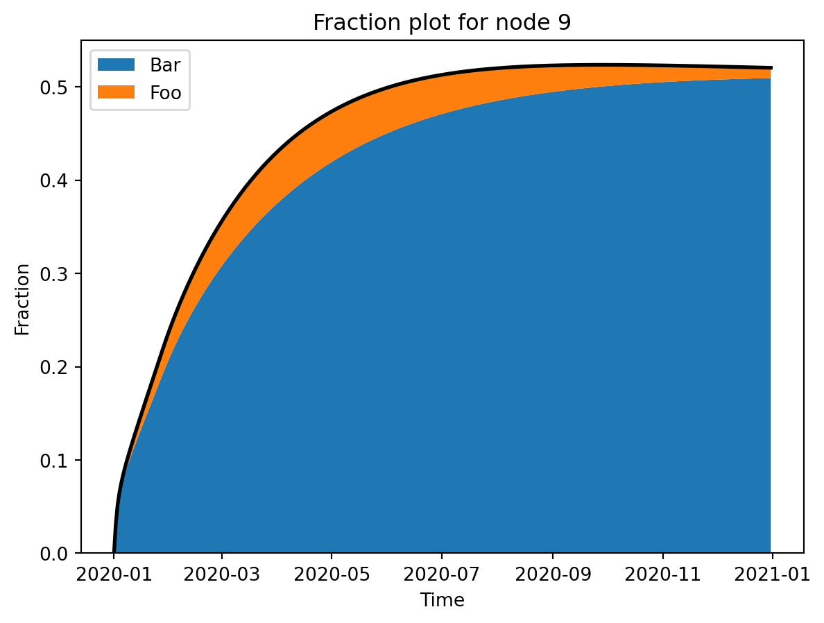
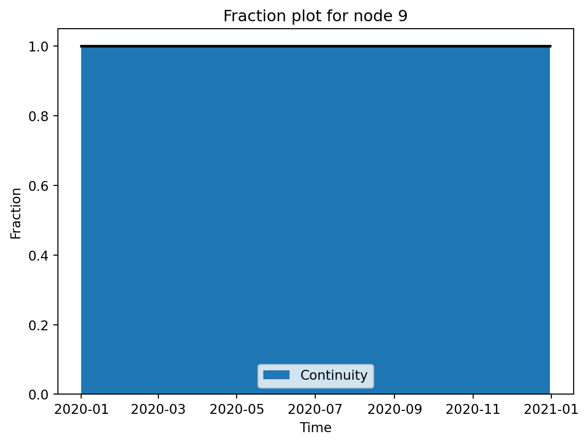
# Plot default tracers (sum to 1), plus custom tracers on node 9
plot_fraction(nmodel, 1)  # default tracers, should add up to 1
plot_fraction(nmodel, 9, ["Foo", "Bar"])  # custom tracers
plot_fraction(nmodel, 9, ["Continuity"])  # mass balance check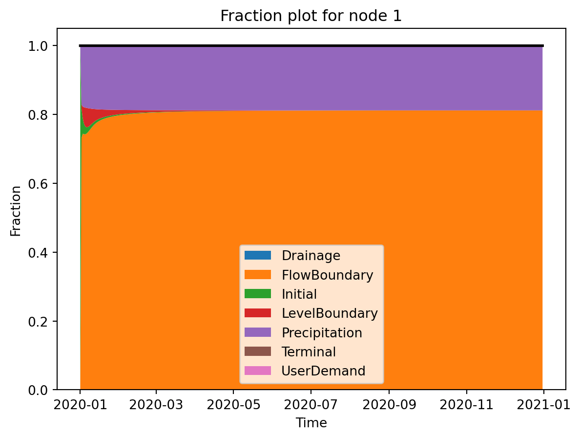

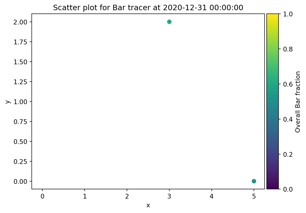
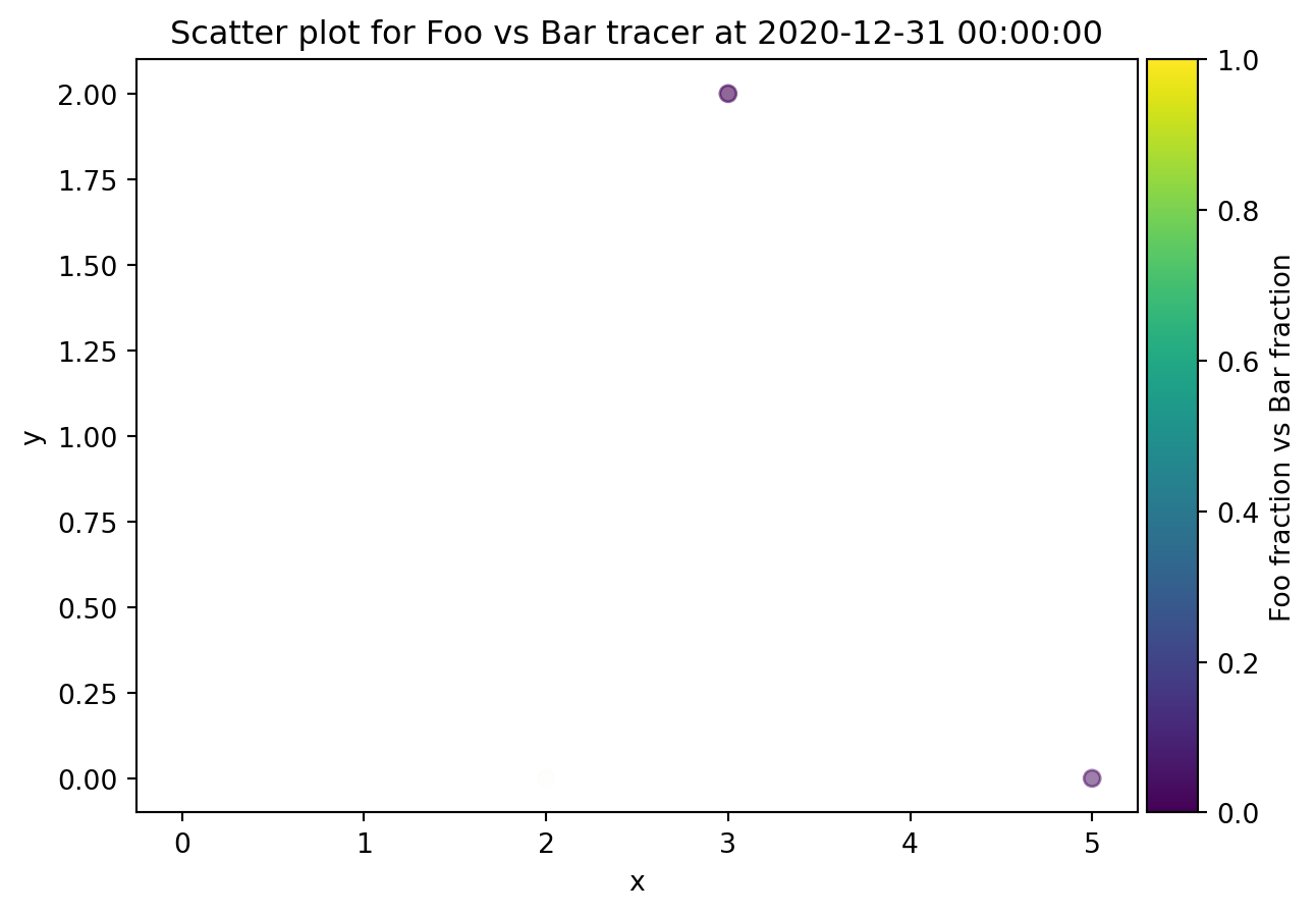
from ribasim.delwaq import plot_spatial

plot_spatial(nmodel, "Bar")
plot_spatial(nmodel, "Foo", versus="Bar")