Basin

The Basin is the central node in each schematization, since it is the only one that stores water. It can exchange water with all other nodes. The connected nodes determine how water is exchanged; the Basin has no flow behavior of its own.

1 Tables

1.1 Static

The Basin / static table can be used to set the static value of variables. The time table has a similar schema, with the time column added. A static value for a variable is only used if there is no dynamic forcing data for that variable. Specifically, if there is either no time table, it is empty, or all timestamps of that variable are missing.

column	type	unit	restriction
node_id	Int32	-	sorted
precipitation	Float64	\(\text{m}/\text{s}\)	non-negative
potential_evaporation	Float64	\(\text{m}/\text{s}\)	non-negative
drainage	Float64	\(\text{m}^3/\text{s}\)	non-negative
infiltration	Float64	\(\text{m}^3/\text{s}\)	non-negative

Note that if variables are not set in the static table, default values are used when possible. These are generally zero, e.g. no precipitation, no inflow. If it is not possible to have a reasonable and safe default, a value must be provided in the static table.

1.2 Time

This table is the transient form of the Basin table. The only difference is that a time column is added. The table must by sorted by time, and per time it must be sorted by node_id.

1.2.1 Interpolation

At the given timestamps the values are set in the simulation, such that the timeseries can be seen as forward filled.

import numpy as np
import pandas as pd
import matplotlib.pyplot as plt
from IPython.display import display, Markdown

np.random.seed(1)
fig, ax = plt.subplots()
fontsize = 15

N = 5
y = np.random.rand(N)
x = np.cumsum(np.random.rand(N))

def forward_fill(x_):
    i = min(max(0, np.searchsorted(x, x_)-1), len(x)-1)
    return y[i]

def plot_forward_fill(i):
    ax.plot([x[i], x[i+1]], [y[i], y[i]], color = "C0", label = "interpolation" if i == 0 else None)

ax.scatter(x[:-1],y[:-1], label = "forcing at data points")
for i in range(N-1):
    plot_forward_fill(i)

x_missing_data = np.sort(x[0] + (x[-1] - x[0]) * np.random.rand(5))
y_missing_data = [forward_fill(x_) for x_ in x_missing_data]
ax.scatter(x_missing_data, y_missing_data, color = "C0", marker = "x", label = "missing data")
ax.set_xticks([])
ax.set_yticks([])
ax.set_xlabel("time", fontsize = fontsize)
ax.set_ylabel("forcing", fontsize = fontsize)
xlim = ax.get_xlim()
ax.set_xlim(xlim[0], (x[-2] + x[-1])/2)
ax.legend()

markdown_table = pd.DataFrame(
        data = {
            "time" : x,
            "forcing" : y
        }
    ).to_markdown(index = False)

display(Markdown(markdown_table))

time	forcing
0.0923386	0.417022
0.278599	0.720324
0.62416	0.000114375
1.02093	0.302333
1.55974	0.146756

As shown this interpolation type supports missing data, and just maintains the last available value. Because of this for instance precipitation can be updated while evaporation stays the same.

1.3 State

The state table gives the initial water levels of all Basins.

column	type	unit	restriction
node_id	Int32	-	sorted
level	Float64	\(\text{m}\)	\(\ge\) basin bottom

Each Basin ID needs to be in the table. To use the final state of an earlier simulation as an initial condition, copy results/basin_state.arrow over to the input_dir, and point the TOML to it:

[basin]
state = "basin_state.arrow"

This will start of the simulation with the same water levels as the end of the earlier simulation. Since there is no time information in this state, the user is responsible to ensure that the earlier endtime matches the current starttime. This only applies when the user wishes to continue an existing simulation as if it was one continuous simulation.

1.4 Profile

The profile table defines the physical dimensions of the storage reservoir of each basin.

column	type	unit	restriction
node_id	Int32	-	sorted
area	Float64	\(\text{m}^2\)	non-negative, per node_id: start positive and not decreasing
level	Float64	\(\text{m}\)	per node_id: increasing

The level is the level at the basin outlet. All levels are defined in meters above a datum that is the same for the entire model. An example of the first 4 rows of such a table is given below. The first 3 rows define the profile of ID 2. The number of rows can vary per ID, and must be at least 2. Using a very large number of rows may impact performance.

node_id	area	level
2	1.0	6.0
2	1000.0	7.0
2	1000.0	9.0
3	1.0	2.2

We use the symbol \(A\) for area, \(h\) for level and \(S\) for storage. The profile provides a function \(A(h)\) for each basin. Internally this get converted to two functions, \(A(S)\) and \(h(S)\), by integrating over the function, setting the storage to zero for the bottom of the profile. The minimum area cannot be zero to avoid numerical issues. The maximum area is used to convert the precipitation flux into an inflow.

1.4.1 Interpolation

1.4.1.1 Level to area

The level to area relationship is defined with the Basin / profile data using linear interpolation. An example of such a relationship is shown below.

fig, ax = plt.subplots()

# Data
N = 3
area = 25 * np.cumsum(np.random.rand(N))
level = np.cumsum(np.random.rand(N))

# Interpolation
ax.scatter(level,area, label = "data")
ax.plot(level,area, label = "interpolation")
ax.set_xticks([level[0], level[-1]])
ax.set_xticklabels(["bottom", "last supplied level"])
ax.set_xlabel("level", fontsize = fontsize)
ax.set_ylabel("area", fontsize = fontsize)
ax.set_yticks([0])

# Extrapolation
level_extrap = 2 * level[-1] - level[-2]
area_extrap = 2 * area[-1] - area[-2]
ax.plot([level[-1], level_extrap], [area[-1], area_extrap], color = "C0", ls = "dashed", label = "extrapolation")
xlim = ax.get_xlim()
ax.set_xlim(xlim[0], (level[-1] + level_extrap)/2)

ax.legend()
fig.tight_layout()

markdown_table = pd.DataFrame(
        data = {
            "level" : level,
            "area" : area
        }
    ).to_markdown(index = False)

display(Markdown(markdown_table))

level	area
0.140387	16.7617
0.338488	27.1943
1.13923	41.1616

For this interpolation it is validated that:

• The areas are positive and are non-decreasing;
• There are at least 2 data points.

This interpolation is used in each evaluation of the right hand side function of the ODE.

1.4.1.2 Level to storage

The level to storage relationship gives the volume of water in the basin at a given level, which is given by the integral over the level to area relationship from the basin bottom to the given level:

\[ S(h) = \int_{h_0}^h A(h')\text{d}h'. \]

storage = np.diff(level) * area[:-1] + 0.5 * np.diff(area) * np.diff(level)
storage = np.cumsum(storage)
storage = np.insert(storage, 0, 0.0)
def S(h):
    i = min(max(0, np.searchsorted(level, h)-1), len(level)-2)
    return storage[i] + area[i] * (h - level[i]) + 0.5 * (area[i+1] - area[i]) / (level[i+1] - level[i]) * (h - level[i])**2

S = np.vectorize(S)

# Interpolation
fig, ax = plt.subplots()
level_eval = np.linspace(level[0], level[-1], 100)
storage_eval = S(np.linspace(level[0], level[-1], 100))
ax.scatter(level, storage, label = "storage at datapoints")
ax.plot(level_eval, storage_eval, label = "interpolation")
ax.set_xticks([level[0], level[-1]])
ax.set_xticklabels(["bottom", "last supplied level"])
ax.set_yticks([0])
ax.set_xlabel("level", fontsize = fontsize)
ax.set_ylabel("storage", fontsize = fontsize)

# Extrapolation
level_eval_extrap = np.linspace(level[-1], level_extrap, 35)
storage_eval_extrap = S(level_eval_extrap)
ax.plot(level_eval_extrap, storage_eval_extrap, color = "C0", linestyle = "dashed", label = "extrapolation")
xlim = ax.get_xlim()
ax.set_xlim(xlim[0], (level[-1] + level_extrap)/2)
ax.legend()

for converting the initial state in terms of levels to an initial state in terms of storages used in the core.

1.4.1.3 Interactive basin example

The profile data is not detailed enough to create a full 3D picture of the basin. However, if we assume the profile data is for a stretch of canal of given length, the following plot shows a cross section of the basin.

import plotly.graph_objects as go
import numpy as np

def linear_interpolation(X,Y,x):
    i = min(max(0, np.searchsorted(X, x)-1), len(X)-2)
    return Y[i] + (Y[i+1] - Y[i])/(X[i+1] - X[i]) * (x - X[i])

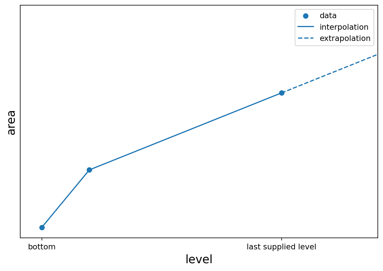
def A(h):
    return linear_interpolation(level, area, h)

fig = go.Figure()

x = area/2
x = np.concat([-x[::-1], x])
y = np.concat([level[::-1], level])

# Basin profile
fig.add_trace(
    go.Scatter(
        x = x,
        y = y,
        line = dict(color = "green"),
        name = "Basin profile"
    )
)

# Basin profile extrapolation
y_extrap = np.array([level[-1], level_extrap])
x_extrap = np.array([area[-1]/2, area_extrap/2])
fig.add_trace(
    go.Scatter(
        x = x_extrap,
        y = y_extrap,
        line = dict(color = "green", dash = "dash"),
        name = "Basin extrapolation"
    )
)
fig.add_trace(
    go.Scatter(
        x = -x_extrap,
        y = y_extrap,
        line = dict(color = "green", dash = "dash"),
        showlegend = False
    )
)

# Water level
fig.add_trace(
    go.Scatter(x = [-area[0]/2, area[0]/2],
               y = [level[0], level[0]],
               line = dict(color = "blue"),
               name= "Water level")
)

# Fill area
fig.add_trace(
    go.Scatter(
        x = [],
        y = [],
        fill = 'tonexty',
        fillcolor = 'rgba(0, 0, 255, 0.2)',
        line = dict(color = 'rgba(255, 255, 255, 0)'),
        name = "Filled area"
    )
)

# Create slider steps
steps = []
for h in np.linspace(level[0], level_extrap, 100):
    a = A(h)
    s = S(h).item()


    i = min(max(0, np.searchsorted(level, h)-1), len(level)-2)
    fill_area = np.append(area[:i+1], a)
    fill_level = np.append(level[:i+1], h)
    fill_x = np.concat([-fill_area[::-1]/2, fill_area/2])
    fill_y = np.concat([fill_level[::-1], fill_level])

    step = dict(
        method = "update",
        args=[
            {
                "x": [x, x_extrap, -x_extrap, [-a/2, a/2], fill_x],
                "y": [y, y_extrap, y_extrap, [h, h], fill_y]
            },
            {"title": f"Interactive water level <br> Area: {a:.2f}, Storage: {s:.2f}"}
        ],
        label=str(round(h, 2))
    )
    steps.append(step)

# Create slider
sliders = [dict(
    active=0,
    currentvalue={"prefix": "Level: "},
    pad={"t": 25},
    steps=steps
)]

fig.update_layout(
    title = {
        "text": f"Interactive water level <br> Area: {area[0]:.2f}, Storage: 0.0",
    },
    yaxis_title = "level",
    sliders = sliders,
    margin = {"t": 100, "b": 100}
)

fig.show()

1.4.1.4 Storage to level

The level is computed from the storage by inverting the level to storage relationship shown above. See here for more details.

1.5 Area

The optional area table is not used during computation, but provides a place to associate areas in the form of polygons to Basins. Using this makes it easier to recognize which water or land surfaces are represented by Basins.

column	type	restriction
node_id	Int32	sorted
geom	Polygon or MultiPolygon	(optional)

1.6 Subgrid

The subgrid table defines a piecewise linear interpolation from a basin water level to a subgrid element water level. Many subgrid elements may be associated with a single basin, each with distinct interpolation functions. This functionality can be used to translate a single lumped basin level to a more spatially detailed representation (e.g comparable to the output of a hydrodynamic simulation).

column	type	unit	restriction
subgrid_id	Int32	-	sorted
node_id	Int32	-	constant per subgrid_id
basin_level	Float64	\(\text{m}\)	sorted per subgrid_id
subgrid_level	Float64	\(\text{m}\)	sorted per subgrid_id

The table below shows example input for two subgrid elements:

subgrid_id	node_id	basin_level	subgrid_level
1	9	0.0	0.0
1	9	1.0	1.0
1	9	2.0	2.0
2	9	0.0	0.5
2	9	1.0	1.5
2	9	2.0	2.5

Both subgrid elements use the water level of the basin with node_id 9 to interpolate to their respective water levels. The first element has a one to one connection with the water level; the second also has a one to one connection, but is offset by half a meter. A basin water level of 0.3 would be translated to a water level of 0.3 for the first subgrid element, and 0.8 for the second. Water levels beyond the last basin_level are linearly extrapolated.

Note that the interpolation to subgrid water level is not constrained by any water balance within Ribasim. Generally, to create physically meaningful subgrid water levels, the subgrid table must be parametrized properly such that the spatially integrated water volume of the subgrid elements agrees with the total storage volume of the basin.

1.7 Concentration

This table defines the concentration(s) of (a) substance(s) for the inflow boundaries of a Basin node.

column	type	unit	restriction
node_id	Int32	-	sorted
time	DateTime	-	sorted per node_id
substance	String		can correspond to known Delwaq substances
drainage	Float64	\(\text{g}/\text{m}^3\)	(optional)
precipitation	Float64	\(\text{g}/\text{m}^3\)	(optional)

1.8 ConcentrationState

This table defines the concentration(s) of (a) substance(s) in the basin at the start of the simulation.

column	type	unit	restriction
node_id	Int32	-	sorted
time	DateTime	-	sorted per node_id
substance	String	-	can correspond to known Delwaq substances
concentration	Float64	\(\text{g}/\text{m}^3\)

1.9 ConcentrationExternal

This table is used for (external) concentrations, that can be used for Control lookups.

column	type	unit	restriction
node_id	Int32	-	sorted
time	DateTime	-	sorted per node_id
substance	String	-	can correspond to known Delwaq substances
concentration	Float64	\(\text{g}/\text{m}^3\)

2 Equations

2.1 The reduction factor

At several points in the equations below a reduction factor is used. This is a term that makes certain transitions more smooth, for instance when a pump stops providing water when its source basin dries up. The reduction factor is given by

\[\begin{align} \phi(x; p) = \begin{cases} 0 &\text{if}\quad x < 0 \\ -2 \left(\frac{x}{p}\right)^3 + 3\left(\frac{x}{p}\right)^2 &\text{if}\quad 0 \le x \le p \\ 1 &\text{if}\quad x > p \end{cases} \end{align}\]

Here \(p > 0\) is the threshold value which determines the interval \([0,p]\) of the smooth transition between \(0\) and \(1\), see the plot below.

import numpy as np
import matplotlib.pyplot as plt

def f(x, p = 3):
    x_scaled = x / p
    phi = (-2 * x_scaled + 3) * x_scaled**2
    phi = np.where(x < 0, 0, phi)
    phi = np.where(x > p, 1, phi)

    return phi

fontsize = 15
p = 3
N = 100
x_min = -1
x_max = 4
x = np.linspace(x_min,x_max,N)
phi = f(x,p)

fig,ax = plt.subplots(dpi=80)
ax.plot(x,phi)

y_lim = ax.get_ylim()

ax.set_xticks([0,p], [0,"$p$"], fontsize=fontsize)
ax.set_yticks([0,1], [0,1], fontsize=fontsize)
ax.hlines([0,1],x_min,x_max, color = "k", ls = ":", zorder=-1)
ax.vlines([0,p], *y_lim, color = "k", ls = ":")
ax.set_xlim(x_min,x_max)
ax.set_xlabel("$x$", fontsize=fontsize)
ax.set_ylabel(r"$\phi(x;p)$", fontsize=fontsize)
ax.set_ylim(y_lim)

fig.tight_layout()
plt.show()

2.2 Precipitation

The precipitation term is given by

\[ Q_P = P \cdot A. \tag{1}\]

Here \(P = P(t)\) is the precipitation rate and \(A\) is the maximum area given in the Basin / profile table. Precipitation in the Basin area is assumed to be directly added to the Basin storage. The modeler needs to ensure all precipitation enters the model, and there is no overlap in the maximum profile areas, otherwise extra water is created. If a part of the catchment is not in any Basin profile, the modeler has to verify that water source is not forgotten. It can for instance be converted to a flow rate and added to a Basin as a FlowBoundary.

2.3 Evaporation

The evaporation term is given by

\[ Q_E = E_\text{pot} \cdot A(u) \cdot \phi(d;0.1). \tag{2}\]

Here \(E_\text{pot} = E_\text{pot}(t)\) is the potential evaporation rate and \(A\) is the wetted area. \(\phi\) is the reduction factor which depends on the depth \(d\). It provides a smooth gradient as \(u \rightarrow 0\).

A straightforward formulation \(Q_E = \mathrm{max}(E_\text{pot} A(u), 0)\) is unsuitable, as \(\frac{\mathrm{d}Q_E}{\mathrm{d}u}(u=0)\) is not well-defined.

A non-smooth derivative results in extremely small timesteps and long computation time. In a physical interpretation, evaporation is switched on or off per individual droplet of water. In general, the effect of the reduction term is negligible, or not even necessary. As a surface water dries, its wetted area decreases and so does the evaporative flux. However, for (simplified) cases with constant wetted surface (a rectangular profile), evaporation only stops at \(u = 0\).

2.4 Infiltration and Drainage

Infiltration is provided as a lump sum for the Basin. If Ribasim is coupled with MODFLOW 6, the infiltration is computed as the sum of all positive flows of the MODFLOW 6 boundary conditions in the Basin:

\[ Q_\text{inf} = \sum_{i=1}^{n} \sum_{j=1}^{m} \max(Q_{\mathrm{mf6}_{i,j}}, 0.0) \tag{3}\]

Where \(i\) is the index of the boundary condition, \(j\) the MODFLOW 6 cell index, \(n\) the number of boundary conditions, and \(\text{m}\) the number of MODFLOW 6 cells in the Basin. \(Q_{\mathrm{mf6}_{i,j}}\) is the flow computed by MODFLOW 6 for cell \(j\) for boundary condition \(i\).

Drainage is a lump sum for the Basin, and consists of the sum of the absolute value of all negative flows of the MODFLOW 6 boundary conditions in the Basin.

\[ Q_\text{drn} = \sum_{i=1}^{n} \sum_{j=1}^{m} \left| \min(Q_{\mathrm{mf6}_{i,j}}, 0.0) \right| \tag{4}\]

The interaction with MODFLOW 6 boundary conditions is explained in greater detail in the the iMOD Coupler docs.